Nicky Pochinkov

*Epistemic Status: Highly Speculative. I spent less than a day thinking about this in particular, and though I have spent a few months studying large language models, I have never trained a language model. I am likely wrong about many things. I have not seen research on this, so it may be useful for for someone to do a real deep dive.*

Thanks to Anthony from the Center on Long Term Risk for sparking the discussion earlier today for this post. Also thanks to conversations with Evan Hubinger ~1 year ago that got me thinking about the topic previously.

Summary

My vague suspicions at the moment are somewhat along the lines of:

• Training an initial model: moderate to low path-dependance
• Running a model: high “prompt-dependance”
• Reinforcement Learning a Model: moderate to high path-dependance.

Definitions of “low” and “high” seem somewhat arbitrary, but I guess what I mean is how different behaviours of the model can be. I expect some aspects to be quite path dependant, and others not so much. This is trying to quantify how many aspects might have path-dependance based on vibe.

Introduction

Path dependence is thinking about the “butterfly effect” for machine learning models. For highly path-dependant models, small changes in how a model is trained can lead to big differences in how it performs. If a model is highly path-dependant, then if we want to understand how our model will behave and make sure it's doing what we want, we need to pay attention to the nitty-gritty details of the training process, like the order in which it's learning things, or the random weights initialisation. And, if we want to influence the final outcome, we have to intervene early on in the training process.

I think having an understanding of path-dependance is likely useful, but have not really seen any empirical results on the topic. I think that in general, it is likely to depend on different training methods a lot, and in this post I will give some vague impressions I have on the path dependance of Large Language Models (LLMs).

In this case, I will also include “prompt-dependance” as another form of “path-dependance” when it comes to the actual outputs of the models, though this is not technically correct since it does not depend on the actual training of the model.

Initial Training of a Model

My Understanding: Low to Moderate Path-Dependance

So with Large Language Models at the moment, the main way they are trained it that you should have a very large dataset, randomise the order, and use each text exactly once. In practice, many datasets have a lot of duplicate data of things that are particularly common (possible example: transcripts of a well-know speech) though people try to avoid this. While this may seem there should be a large degree of path dependance, my general impression is that, at least in most current models, this does not happen that often. In general, LLMs can tend to struggle with niche facts, so I would perhaps expect that in some cases it learns a niche fact that it does not learn in another case, but the LLMs seems to be at least directionally accurate. (An example I have seen, is that it might say “X did Mathematics in Cambridge” instead of “X did Physics in Oxford”, but compared to possibility space, it is not that far.)

I suspect that having a completely different dataset would impact the model outputs significantly, but from my understanding of path dependance, this does not particularly fall under the umbrella of path dependance, since it is modelling a completely different distribution. Though even in this case, I would suspect that in text from categories in the overlapping distribution, that the models would have similar looking outputs (though possibly the one trained on only that specific category could give somewhat more details.)

I also think that relative to the possibility space, most models are relatively stable in their possible options for outputs. Prompting with the name of the academic paper on a (non-fine-tuned) LLM can understand it is an academic title, but can follow up with the text of the paper, or the names of the authors and paper, followed by other references. or simply titles of other papers. I tried this briefly on GPT-3 (davinci) and GPT-NeoX, and both typically would try to continue with a paper, but often in different formats on different runs. What seemed to matter more to narrow down search space was what specific punctuation was placed after the title, such as , “ –” or “ ,”. (More on this in the next section)

I would guess that things like activation functions and learning rate parameters would have difference in how “good” the model gets, but for different models of the same “goodness”, and likely the internals will look different, but I doubt there is much that difference in the actual outputs.

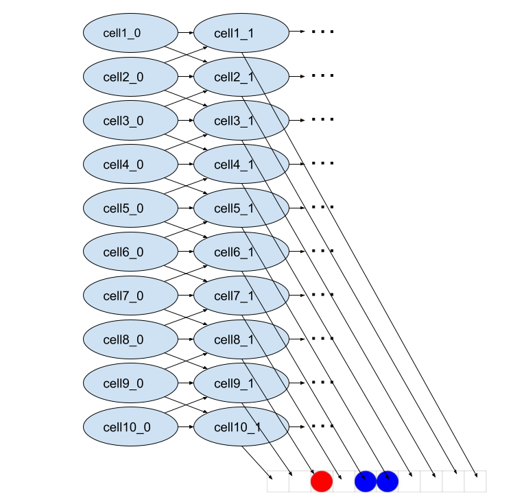
This is partially motivated by the Simulators model of how LLMs work. While imperfect, it seems somewhat close, and much better description than any sort of “agentic” model of how LLMs work. In this model, the essential idea is that LLMs are not so much a unified model trying to write something, but rather, the LLM is using the information in the previous context window to try to model the person who wrote the words, and then simulate what they would be likely write next. In this model, the LLM is not so much learning a unified whole of a next token predictor, but rather it is building somewhat independant “simulacra” models, and using relevant information to update each of them appropriately.

So the things I would expect to have a moderate impact are things like:

• Dataset contents and size
• Tokenizer implementation
• Major architectural differences (eg: RETRO-like models)

And some things I think are less impactful to the output:

• Specific learning rate/other hyperparameters
• Specific Random Initialisation of the Weights/Biases
• Dataset random ordering

Though this is all speculative, I think that if you have a set of 3 models trained on the same dataset, possibly with slightly different hyperparameters, that the output to a well specified prompt would be pretty similar for the most part. I expect the random variations from non-zero temperature would be much larger than the differences due to the specifics of training for tasks similar to the distribution. I would also expect that for tasks that have neat circuits, that you would pretty much find quite similar transformer circuits for a lot of tasks. 

It is possible however, that since many circuits could use the same internal components, then there might be “clusters” of circuit space. I suspect however that the same task could be accomplished with multiple circuits, and that some are exponentially easier to find than others, but there might be some exceptions where there are two same-size circuits that accomplish the same task, or

Some exceptions where I might expect differences:

• Niche specific facts only mentioned once it the dataset at the start vs the end.
• The specific facts might be different for models with lower loss.
• The specific layers in which circuits form.
• Formatting would depend on how the data is scraped and tokenized.
• Data way outside the training distribution. (for example, a single character highly repeated, like “.................”)

So I think it does make a difference how you set up the model, but the difference in behaviour is likely much smaller compared to which prompt you choose. I also suspect most that of the same holds for fine-tuning (as long as they do not use reinforcement learning).

Running a (pre-trained) Model

My Understanding: High “Prompt-Dependance”

When it comes to running a model however, I think that specific input dependance is much higher. This is partially from just interacting with models some what, and also from other people. Depending on the way your sentences are phrased, it could think it is simulating one context, or it could think it is simulating another context.

For example, if you could prompt it with two different prompts:

• “New Study on Effects of Climate Change on Farming in Europe”
• “Meta-analysis of climate impacts and uncertainty on crop yields in Europe “

While both are titles to things answering the same information, one could get outputs that differ completely, since the first would simulate something like a news channel, and the latter might sound more like a scientific paper, and this could result in the facts it puts out to be completely different.

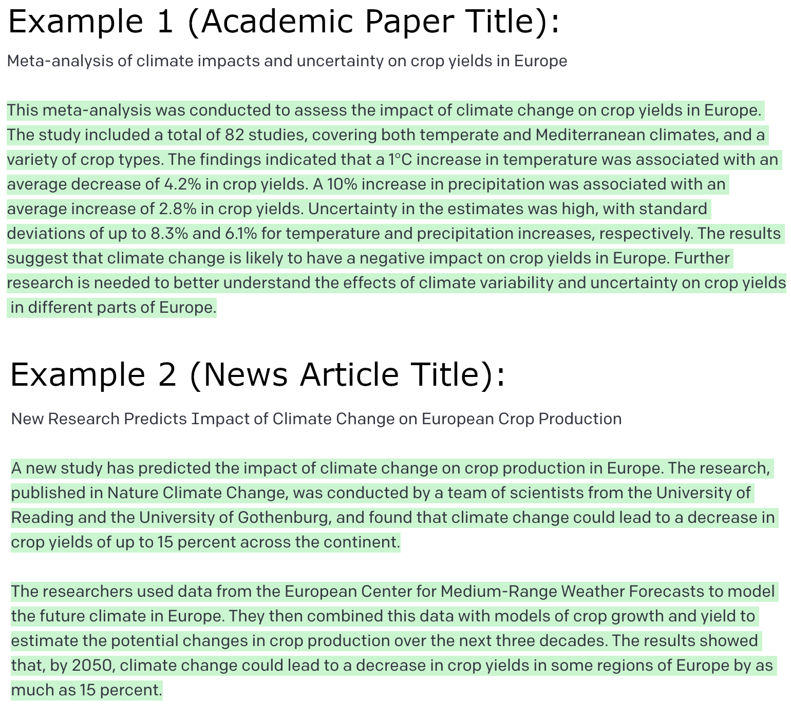
Examples of both the facts and styles being different with different prompts for the same information. Examples run on text-davinci-003

From talking to people who know a lot more than me about Prompt Engineering, even things like formatting newlines, spelling, punctuation and spaces can make a big difference to these sorts of things, depending on how it is formatted in the datasets. As described in the previous section, giving an academic title with different punctuation will make a big difference to the likely paths it could take.

This is one of the main reasons I think that initial training has relatively little path dependance. Since the prompting seems make such a large difference, and seems to model the dataset distribution quite well, I think that the majority of the difference in output is likely to depend almost exclusively on the prompts being put in.

Fine-Tuning LLMs with Reinforcement Learning (RL)

My Understanding: Moderate to High Path Dependance

My understanding of RL on language models is that the procedure is to take some possible inputs and generate responses. Depending on the answers, rate the outputs and backpropagate loss to account for this. Rating could be done automatically (eg: a text adventure game, math questions) or manually (eg: reinforcement learning with human feedback).

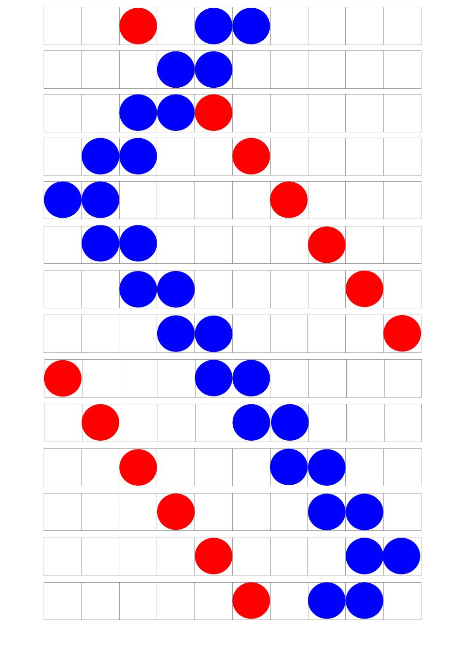
I have not yet done any reinforcement learning on language models in particular, but other times I from implementing RL in other settings I have learned it can be quite brittle and finicky. I think that RL learning on LLMs seems likely to also suffer from this, and that different initial answers could likely sway the model quite quickly. Since the model is generating it's own training set, the initial randomly-generated responses may happen to have somewhat random attributes (eg: tone/spelling/punctuation) be corellated with the correctness of the outputs, and this could lead to the model in the next epoch to reinforce cases where it uses these random attributes more, and so it could get reinforced until the end.

As an toy example, one could imagine getting 10 outputs, 2 of which are “correct”, and happen both to have British English spelling. In this case, the model would learn that the output needs to be not only correct, but have British English spelling. from then on, it mostly only answers in British English spelling, and each time it reinforces the use of British English spelling.

While this doesn't seems like a particularly illustrative example, the main thing is that minor differences in the model are amplified later on in training.

Is suspect however, that there exist RL fine tuning tasks that are less path-dependant. Depending on the reinforcement learning, it could make it so that the model is more or less “path-dependant” on the specific inputs it is prompted with, at least within the training distribution. Outside the training distribution, I would expect that the random amplified behaviours could be quite wild between training runs.

Conclusion.

Again, this writeup is completely speculative on not particularly based on evidence, but from intuitions. I have not seen strong evidence for most of these claims, but I think that the ideas here are likely at least somewhat directionaly correct, and I think that this is an interesting topic people could potentially do some relatively informative tests relatively easily if one has the compute. One could even just look at the differences between similarly performing models of the same size, and come up with some sort of test for some of these things.

There might be existing studied into this which I have missed, or if not, I am sure there are people who likely have better intuitions than me on this, so I would be interested in hearing them.

References

“Path Dependence in ML Inductive Biases”, by Vivek Hebbar, Evan Hubinger

“Simulators”, by janus

“A Mathematical Framework for Transformer Circuits”, by Nelson Elhage, Neel Nanda, Catherine Olsson, et al.

​Produced as part of the SERIMATS Program 2022 Research Sprint under John Wentworth

Introduction

The gold-standard of interpretability in ML systems looks like finding embeddings of human-identifiable concepts in neural net architectures, and being able to modify, change, and activate them as we wish. The first hurdle is identification of these concepts. We propose that it may be easier to identify simpler concepts in simpler models, and use these to bootstrap to more complex concepts in more intricate models.

To this end, we first propose a definition of what it means for a concept to be present in a model. Then we investigate how we can identify similar concepts across different models. We begin by demonstrating these definitions and techniques in a simple example involving Bayes nets.

We then train two autoencoders (small and large) on the FashionMNIST dataset. We choose some latent concepts that humans would use to represent shoes (shoe height and shoe brightness) and see whether these human concepts can be transferred to the models, and how the models' representations relate.

A simple example

Simple Environment

First we construct a simple environment:

• There are 10 cells.
• Each cell can contain nothing, a blue circle, a red circle, or both.
• There is one red circle.
  • The red circle moves 1 right each timestep.
  • If the red circle cannot move right, it moves to the leftmost cell.
• There are two adjacent blue circles.
  • The blue circles move 1 left or 1 right each timestep. 
  • If a blue circle reaches the environment's edge, both their directions change.
• If a cell contains a red circle and a blue circle, it shows only a blue circle.

A sample is given below:

Two Models of this Environment

We model the evolution of this environment using two different Bayes nets. Each Bayes net reflects a different way of viewing this environment corresponding to:

• An object centric model
• A local-state centric model

Object Centric Model (Model 1)

The object centric model tracks 3 latent variables corresponding to the object-level description of where the blue and red circles are and in which direction the blue circles are moving at a given timestep:

• blue location (taking values in \(\{0,1,2,3,4,5,6,7,8,9\}\))
• red location (taking values in \(\{0,1,2,3,4,5,6,7,8,9\}\))
• blue velocity (taking values in \(\{-1,1\}\))

It also has 10 observational variables given by the 10 cells, which take values in \(\{\text{blank},\text{blue},\text{red}\}\).

This is represented by the following Bayes net (each column being a new timestep):

So this Bayes net has a latent space given by the set \(\{0,1,2,3,4,5,6,7,8,9\}^{2}\times\{-1,1\}\), and the state displayed at timestep 2 in the above diagram would have (assuming blue is moving right) latent representation \((2,4,1)\).

Local-State Centric Model (Model 2)

The local-state centric model treats each cell as having a local state corresponding to

• Whether the cell contains a red circle
• Whether the cell contains a blue circle
  • If the cell contains a blue circle, which direction the blue circle is moving in

So each cell can be in one of six possible states:

• No Red, No Blue - \(0\)
• Red, No Blue - \(1\)
• No Red, Blue moving left - \(2\)
• Red, Blue moving left - \(3\)
• No Red, Blue moving right - \(4\)
• Red, Blue moving right - \(5\)

And this is represented by the Bayes net:

So the latent space of this Bayes net consists of tuples from the set \(\{0,1,2,3,4,5\}^{10}\), and the state displayed at timestep 1 would have (assuming blue is moving right) latent representation \((0,0,1,0,4,4,0,0,0,0)\).

Definitions

Now that we have an environment and two simple models to refer to, let's define some notions that will be useful:

A latent concept is an abstract concept which changes across the training data. Some examples in the above environment: 'blue direction,' 'location of the blue circle,' 'location of all three circles,' and 'state of the 3rd cell.' (Due to the simple nature of the above environment, all of these latent concepts take values in discrete sets, but latent concepts can be continuous as well.)

Relationship components take latent concepts as input, and output how these change other latent concepts in the model. They do this by representing operations or functions that are constant across the training data. In the above example, this might be 'the red circle always moves right' or 'the blue circles bounce off the edge.'

A latent concept identifier takes as input a vector in the latent space of a model, and outputs the value of the latent concept being measured.

These concepts at work in Bayes nets

We will choose 'blue velocity' as our latent concept and establish a latent concept identifier for blue velocity in the object centric Bayes net. Then we want to use this latent concept identifier to communicate this latent concept from the object centric latent space to the local-state centric latent space and hence derive the latent concept identifier in this new latent space. 

The latent concept identifier function for blue velocity in the object centric Bayes net is obvious by inspection, it is simply:

\(\begin{equation}  f_{1}:\{0,1,2,3,4,5,6,7,8,9\}^{2}\times\{-1,1\} \to \{-1,1\} \end{equation}\)

such that

\(f_{1}\big((a,b,c)\big) = c\),

since this concept is represented directly in the third coordinate of the latent space.

The second latent space stores this same concept in a noticeably more indirect and distributed way, and the latent concept identification function is correspondingly more complex.\(\)\(\)\(\)

\(f_{2}:\{0,1,2,3,4,5\}^{10}\to\{-1,1\}\)

such that

\(f_{2}(z)=\begin{cases} 1,  &\text{if any coordinate in $z$ contains a 4 or 5,}\\ -1, &\text{if any coordinate in $z$ contains a 2 or 3.}  \end{cases}\)

This function would be easy to learn from example data using a decision tree or neural net. This would be done by generating observation sequences using the object centric Bayes net, then obtaining the corresponding latent state using the local-state Bayes net, and labelling it using the object-centric concept identifier and latent state.  The process of learning this function constitutes the transferring of the latent concept from the first latent space to the second latent space which was what we hoped to achieve. 

The complete-data limit

\(\)We now take the general method sketched out in the example above, and formalize it. We aim to show that for 2 models, when we can compare the latent concepts across all possible inputs to the models, we can perfectly communicate latent concepts from one model to another.

Let's define:

• A set of observations \(\)\(O\), in humans this is the set of all possible sequences of sense-data over a lifetime, in the Bayes net example above it's \(\{\text{blank, red, blue}\}^{10 \times \text{max_timesteps}}\).
• Two spaces \(L1\) and \(L2\) \(\)which represent the latent spaces of two world models. 
• Two functions, \(l1\) and \(l2\), to represent each world model. Each function maps observations to latent states, \(l_i: O \to L_i\).  Assume that these world models were trained as generative models to predict any part of the observation given any other part of the observation, so it uses the latent space \(L_i\) to store any information relevant to predicting any potential observation.

Now we have a concept, say “blue velocity”, which we define using a function \(c_1 : L_1 \to \{-1,1\}\). 

Our goal is to successfully communicate a concept from one model to the other. In other words, to discover the function \(c_2: L_2 \to \{-1,1\}\), such that:

\(\forall o \in O, c_1(l_1(o)) = c_2(l_2(o))\)

If we assume \(l_2\) is invertible.^[1]^ 

Then we can define \(c_2\) as:

\(c_2(z) := c_1(l_1(l_2^{-1}(z))))\)  for any \(z \in L_2\).

A similar approach to the above can be used to learn a latent concept identifier that is invertible, i.e. we can use it to manipulate the belief state of the world model. In that case we need to also iterate over possible changes to latent state 1 which match the predictions made by world model 2 when the relevant latent variable is changed.

Variational Autoencoders (VAEs) trained on FashionMNIST

Now we consider a more complex example involving neural nets. We train two variational autoencoders on the FashionMNIST dataset. A variational autoencoder is made up of two components: an encoder and a decoder. The encoder is trained to take in an image and map it to a point in an \(n\)-dimensional latent space. The decoder is simultaneously trained to take these points in the latent space, and reconstruct an image that minimises binary cross-entropy loss between the actual image and what the decoder predicts the image to look like from knowing where the encoder sends it.

VAE FashionMNIST representations

Below are two plots of the latent spaces of variational autoencoders trained with a 2D latent space:

We can see that there are regions of the space that correspond to concepts we might use ourselves to represent fashion items. For example, the top left region in the first latent space, and bottom right region in the second latent space are both 'shoe-regions' in their respective latent spaces. And they seem to be clustered in a fairly sensible way!

There are also regions of these latent spaces that clearly do not correspond to ways we would think about fashion items: an example that occurs in almost every latent space we generated is t-shirts turning into pants, and we can see that both latent spaces store weird half t-shirt, half pants images.

Therefore, we're not looking for every concept that the autoencoder uses to represent fashion items to be analogous to human representations of fashion items. But we are looking for the reverse implication to hold: that human representations of fashion items will have an analogous representation in these latent spaces. Moreover, this holds only for local concepts since global concepts like “formality of fashion items” will not be learnt by the autoencoder, but we would expect local concepts like 'height of shoe' or 'brightness of shirt' to be learnt.

VAEs with Higher Dimensional Latent Spaces

We train two slightly different VAE models of different sizes, a smaller and a larger one. Each model has 20 latent space dimensions, but after training we found that a smaller number of dimensions are used in practice. The number of dimensions used was fairly consistent between different runs. For the smaller model, usually only 5 were used (though sometimes 6). For the larger model, usually 10 were used (sometimes 9). Increasing the number of dimensions in the latent space also had little effect on the number of dimensions the model learns to use.

We use these VAEs to encode two artificially whitened out shoes, and then decode them to see where they get sent. The first whitened out shoe was obtained by selecting a shoe from the dataset, and rounding all the pixel values. The second shoe was obtained by manually adding two white pixels on top of this shoe. Our hope was that this would eliminate other variables (e.g. texture) that might interfere with how the VAEs encode shoes, and that thereby we could determine a vector along which 'shoe height' is varying. 

Shoe encodings (and decodings)

Regular size shoe, and what the model generates from its encoding:

Shoe +2 pixels to height, and what the model generates from its encoding:

Does this give us a vector corresponding to shoe height?

We took this vector along which (we hope) shoe height was varying, normalized it, and plotted images at different points along this vector (taking the origin to be the first encoded shoe) and obtained:

This movement in latent space locally corresponds to shoe height. When we extrapolate far enough in any direction, it will ultimately reach a region of latent space which does not correspond to any human-interpretable concept (c.f. the bottom left region of the two dimensional example latent spaces), so this local behaviour is the best we could hope for.

Now let's vary the same vector about an example of a real encoded shoe. This should show to what extent this direction corresponds to shoe height (although VAEs map concepts non-linearly, so it will be at best a good local approximation of increasing shoe height):

And again it does seem to correspond (roughly) to shoe height.

Larger VAE

We then apply this procedure to the larger VAE, and generate corresponding images that (we hope) vary just in shoe height. In this VAE, however, moving along the height vector also increases brightness. (especially noticeable in the second image below, but present in both):

Orthogonal vectors in latent space

We then investigate whether we can separate the model's learnt concept for brightness from its learnt concept for shoe height:

Varying an image along the vector for “brightness” for the smaller VAE 

Varying an image along the vector for “brightness” for the larger VAE 

Some brief attempts were tried by first getting a vector for brightness and then a vector orthogonal to this (using Gram-Schmidt), but this didn't quite work. Depending on how one increased brightness, one could get a vector that is not orthogonal to shoe height. For the larger VAE,  moving along the brightness vector, the shoe gets both brighter and taller than in the shoe height direction – our orthogonalization attempts unfortunately did not end up working.

Directions worth further research

• The sample efficiency of learning a latent concept identifier should depend on the similarity of the abstractions used by each model.  Can we demonstrate this? Can we make progress on this by assuming some version of the natural abstraction hypothesis?
• How do we formalize learning latent concept identifiers to cases where we are transferring from a better model to a worse model of the world (i.e. when \(l_2\) is not invertible)?
• How do we extend learning latent concept identifiers to cases where both models are imperfect in different ways: where one model is better at predicting some types of observations but is beaten on others?
• Can we isolate independent directions in the latent space of variational autoencoders that actually represent identifiable concepts orthogonally?
• Can we find similar behaviour in larger autoencoders of more complex datasets? Will increasing the number of parameters and complexity of data serve to make represented concepts more human-identifiable, or less?

1. ^^^

   Note that this is a strong assumption, it implies that any observation sequence leads to a unique “belief state” about the world. I.e. it's a lossless representation of the world. The assumption makes sense for perfectly modelled deterministic environments.

A product of a SERI MATS research sprint (taking 1.5 weeks).

Cannot yet assign positively to animal or vegetable kingdom, but odds now favour animal. Probably represents incredibly advanced evolution of radiata without loss of certain primitive features. Echinoderm resemblances unmistakable despite local contradictory evidences. Wing structure puzzles in view of probable marine habitat, but may have use in water navigation. Symmetry is curiously vegetable-like, suggesting vegetable’s essentially up-and-down structure rather than animal’s fore-and-aft structure …

Vast field of study opened … I’ve got to dissect one of these things before we take any rest.

—H. P. Lovecraft, At the Mountains of Madness

Introduction

This is our MATS research-sprint team's crack at working towards the True Name (the formalization robust to arbitrary amounts of adversarial optimization power) of a model's “internal machinery.”

Some weights and neurons in a model are essential to its performance, while other weights and neurons are unimportant. Our idea is that, ontologically, the True Name of a model's internal machinery is its subnetwork of important weights and neurons — its “skeleton.” This subnetwork is still a (sparser) model, but hopefully a far more interpretable model than the original.

What makes this a theoretically interesting True Name is our theory's intersection with the theory of “broad peaks” ('Rashomon ridges) in the loss landscape of overparametrized models. Rashomon ridges suggest that different overparametrized models, trained to optimality on the same task, will share a single skeleton. Furthermore, Rashomon ridges suggest a means to compute the shared skeleton of that class of models.

We were able to execute our pruning algorithm effectively by leaning on \(L^1\) regularization. \(L^1\)-regularization-plus-pruning-extremely-small-weights shrunk models significantly while never unacceptably varying loss or accuracy. However, the models we trained did not obviously converge to skeletons, as measured by their losses on an off-distribution task. This means something is up with one or more of our premises: (1) Rashomon ridges are not so naively traversable and/or (2) our argument for shared internal machinery amongst models on a Rashomon ridge fails.

Loss Landscapes and Rashomon Ridges

A loss landscape is a geometric representation of how good various models are at a task.

An example loss landscape

\((x, y)\) coordinates in the loss landscape above represent models with two parameters, \(x\) and \(y\). Thus, the two horizontal dimensions of the loss landscape represents a model space — every point in that plane is a possible model you could have. For larger models, their model spaces will have correspondingly more dimensions.

The vertical dimension \(z\) in the loss landscape represents how good the model \((x, y)\) is at a given task. (Whether we represent this as higher-is-better or lower-is-better is immaterial.) In the above loss landscape, then, every point \((x, y, z)\) represents a model and its loss. SGD initializes at some random point in that landscape, and rolls downhill from there, “reaching optimality” once the model settles into some rut.

A Rashomon manifold (or Rashomon ridge) is a large flat plateau in the loss landscape of overparameterized optimal models. It has been conjectured that, and disputed whether, these overparametrized models trained to optimality land on Rashomon manifolds that encompass all optima. Rashomon ridges are conjectured to widen and narrow periodically, and to run through all the optima in overparameterized model spaces. (The idea here is that overparameterized models have a lot of free, superfluous parameters, and that these free dimensions in model space almost certainly allow all optima in the high-dimensional loss landscape to intersect each other.)

Skeletons

One can imagine an optimal model additionally barnacled with superfluous neurons, where all the weights in the superfluous neurons are zero. These zeroed-out neurons don't help or hurt the model's loss — they just sit there, inert. We can therefore permanently prune these zeroed-out neurons from the model without changing the model's loss.

Consider only those weights and neurons that would counterfactually tank a model's loss were they pruned (ignoring the irrelevant weights and neurons in the model). Call this sparse subnetwork of important weights and neurons the model's skeleton. 

Because this subnetwork is plausibly much smaller than the original network, it will be correspondingly easier to interpret with existing techniques. The challenge now lies, of course, in finding an arbitrary optimal model's skeleton.

Skeleton Hunting

Functioning Machinery under Continuous Deformation

Overparametrized models trained to optimality (possibly) sit on a Rashomon ridge of related models. When you move from one model to its neighbor on the Rashomon ridge, you're looking at some small change in model weights that doesn't change the model's loss. So traveling around on the Rashomon ridge means seeing a model continuously morph, Shoggoth-like, into models with equivalent losses via small changes. You can morph the model in all sorts of ways by moving around the Rashomon ridge, but you never (1) discontinuously morph it or (2) hurt its loss.

Because all these changes are small and the loss is held constant, whatever machinery the model is using internally cannot be being radically revised. If step sizes were large, we could jump from a model that succeeds one way to a model that succeeds in a very different way, stepping over a valley of hybrid, non-functional models in between. If model losses were allowed to vary, then travel through the valley of non-functional hybrid models would be permitted. But when step sizes are kept small, so that the model is only ever being altered in small ways, and when losses are held constant or nearly constant, keeping the model on a flat Rashomon plateau, we bet the model's internal machinery cannot change.^[1]^

We leverage the fact that all the models of a Rashomon ridge then share their internal machinery — “skeleton” — to actually construct the skeleton of an arbitrary model on that ridge! What we're after is an exposed skeleton: the sparsest model on the Rashomon ridge. Because all models on the ridge share a skeleton, locating this exposed-skeleton model gives us insight into the inner workings of all other models on the ridge.

Our method is to (1) apply \(L^1\) regularization to the optimal models, and then (2) prune all the extremely small weights of those models. We found that this surprisingly did not significantly alter model losses or accuracy, and resulted in substantially smaller, equivalently powerful models — our skeletons.

\(L^1\) Regularization and Pruning

How can we prune in a manner that never significantly moves the model's loss? A common way to train a model simultaneously towards optimality and low-dimensionality (a model with many zero weights) is\(L^1\) regularization. If \(f(w): W \to \mathbb R\) denotes the loss function (on the weight space \(W\)) given by the training dataset, then\(L^1\)regularization denotes the technique of applying SGD not on \(f(w)\) itself, but on the modified loss function

\[f_{\lambda}(w)=(1-\lambda )f(w)+\lambda \sum_i |w_i|\]

for some \(0<\lambda<1.\) Here, the function \(w \mapsto \sum_i |w_i|\) is the\(L^1\) norm of the weight vector \(w\). The weight \(\lambda\) should ideally be not so small that the regularization has essentially no effect, but not so large that training ceases to care about model optimality.

\(L^1\)regularization drives many weights to decrease in magnitude to zero while maintaining an optimal model. Intuitively, \(L^1\) regularization reduces the magnitude of all the weights by a fixed positive amount (corresponding to the slope of the absolute value function), until weights are set to zero.

L1 regularization minimizes the sum of the absolute values of all the model's weights.

Once \(L^1\) regularization has driven down the weights sufficiently, we permanently prune out those weights.

Experimental Results

Our plan was to start with two different optimal models, prune each of them, and probe whether they have become more similar as a result. To do so, we need a way to measure the similarity of two neural-net models. No canonical measure of neural network similarity currently exists, however. Given this, we were inspired by Ding et al. to first look at the comparative behavior of the two models out-of-distribution. This is because neural nets which are canonically similar inside of their respective black boxes would as a consequence behave similarly outside of them. That is, they would have similar behavior on datasets other than the training dataset. 

We had predicted that our two models, trained to optimality on the same task, would end up as the same pruned model (or at least highly similar in their network structures). This would be surprising, and not something that other theories would wager would happen!

We trained two separate models to optimality at the CIFAR10 image classification task (sorting 32x32 images of frogs, planes, trains, etc.). We next \(L^1\) regularized those two optimal models, so as to incentivize them to drive down the sum of their weights. This never substantially changed their losses or accuracy. Finally, we heavily pruned the two regularized models, permanently deleting all weights below the threshold of 0.05, which we found to not significantly reduce accuracy.

Deploying our image models after pruning them via the above light-\(L^1\)-regularization-and-pruning on an entirely separate MNIST classification task. Our models had previously inhabited a world of 32x32 images of frogs and planes and so on, and so had never before encountered handwritten digits. Thus, the handwritten digits task probes their out-of-distribution behavior, which isn't constrained by the optimality criterion on in-distribution performance. If the models were the same or were becoming the same as a consequence of pruning, then this unconstrained external comparison of similarity would reveal that. Two truly identical models will behave identically, on and off distribution.

We obtained a variety of optimal models, each of which was obtained by applying a different pruning strategy to either Model 1 or Model 2. Then, for every pair of these pruned models, we computed the cosine similarity of their prediction vectors on the out-of-distribution MNIST dataset 

\[\text{CosineSimilarity}(A,B)=\frac{A\cdot B}{||A||\cdot||B||}\]

Here's our plot of the cosine similarity of each pair of model's behavior on the out-of-distribution MNIST task:

Model indices run from top to bottom and from left to right. The white squares are the most similar, and the dark squares are the least similar.
0: Model 1, trained for 200 epochs, unpruned 
1: Model 1, L1 regularization with 1e-6 for 200 epochs 
2: Model 1, L1 regularization with 1e-6 for 400 epochs 
3: Model 1, L1 regularization with 3e-6 for 300 epochs 
4: Model 1, L1 regularization with 1e-5 for 100 epochs 
5: Model 1, L1 regularization with 1e-5 for 300 epochs 
6: Model 2, trained for 200 epochs, unpruned 
7: Model 2, L1 regularization with 1e-6 for 200 epochs 
8: Model 2, L1 regularization with 1e-6 for 400 epochs 
9: Model 2, L1 regularization with 3e-6 for 300 epochs 
10: Model 2, L1 regularization with 1e-5 for 100 epochs 
11: Model 2, L1 regularization with 1e-5 for 300 epochs 
12: Model trained with L1 Regularization 1e-6, 200 epochs 
13: Model trained with L1 Regularization 1e-6, 300 epochs 
14-27: same with weights below 0.01 removed
28-41: same with weights below 0.02 removed 
42-55: same with weights below 0.05 removed

Unsurprisingly, pruning from a higher weight threshold more dramatically altered out-of-distribution model behavior than pruning only smaller weights did. More epochs spent in \(L^1\) regularization produced smaller pruned models with similar out-of-distribution behavior to their unpruned originals.

Our various models all had similarly varied out-of-distribution behavior — generally, a cosine similarity of >0.6 with each other on MNIST. Model 51 was our only exception to this rule. As you can see above, model 51's cosine similarity of <0.6 (in black/purple) stands out on the plot, and 51 curiously suffered from a relatively degraded loss on CIFAR10 (curiously, because models regularized harder and pruned at the same threshold did not suffer loss degradation in the same way).

Tragically, then, our data does not suggest that models on a Rashomon ridge converge to a shared skeleton under\(L^1\) regularization plus pruning.

1. ^^^

   The Worry from “Multi-Skeletal” Models:

   Consider models with “two skeletons” that each effectively and independently contribute to the loss, but that pass through lossy channels on their way out of the model. This model could smoothly shift between its substantially different skeletons by shifting weight contributions from one skeleton over to the other, such that loss is smoothly preserved. If examples of this exist, then our premise that all optimal models on a Rashomon ridge share a single skeleton would be false.

   One reason to worry less about this “multi-skeleton” failure case of our theory is that the trained models we're looking at are already trained to optimality. If the models are optimal, then it shouldn't be that they have a well of optimization power to draw from to keep their loss constant. They can't have a whole second skeleton, held in reserve. Instead, the models should be doing as well as is possible with any small change — “multi-skeletal” models would be holding back and so would be able to fall further in the loss landscape. This implies that all the machinery of an optimal model is actively in use, and thus that every optimal model is “mono-skeletal.”